Best practices for layouts

In this set of tutorials, we will cover several techniques that improve code readability and reusability, as well as highlight several functions provided by the qnngds.utilities module

Use of DeviceSpec and functools.partial

In this tutorial, we will cover an example that illustrates why using the DeviceSpec pattern along with functools.partial is essential for keeping code readable, reusable, and maintainable by comparing two ways to implement the code used in _custom_circuit.

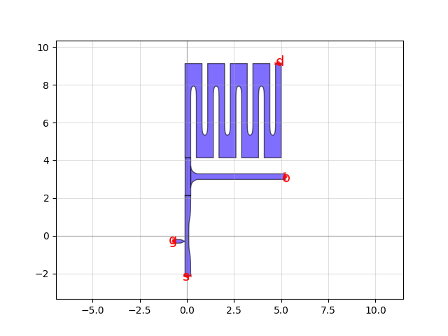
First will be the example circuit without using DeviceSpec or functools.partial. This particular example is a canonical example of the type of problem one runs into when trying to compose many simple devices into a circuit. Now imagine the complexity if you are integrating this subcircuit into another, larger circuit and want to change the arguments between different instances of this subcircuit.

import qnngds as qg
from qnngds import Device
from qnngds.typing import LayerSpec
import phidl.geometry as pg
from phidl import quickplot as qp


def ntron_meander_complicated(
    ntron_choke_w: float = 0.03,
    ntron_gate_w: float = 0.2,
    ntron_channel_w: float = 0.2,
    ntron_source_w: float = 0.3,
    ntron_drain_w: float = 0.3,
    ntron_choke_shift: float = -0.3,
    meander_width: float = 0.2,
    meander_pitch: float = 0.6,
    meander_size: tuple[int | float | None, int | float | None] = (5, 5),
    meander_num_squares: int | None = None,
    meander_turn_ratio: int | float = 4,
    meander_extend_terminals: bool = True,
    meander_terminals_same_side: bool = False,
    tee_size: tuple[float, float] = (4, 2),
    tee_stub_size: tuple[float, float] = (2, 1),
    tee_taper_type: str | None = "fillet",
    tee_taper_radius: float | None = None,
    num_pts: int = 50,
    layer: LayerSpec = (1, 0),
) -> Device:
    """nTron with meander on drain

    Returns: nTron with connected meander and tee
    """
    D = Device("ntron_meander")

    ntron = D << qg.devices.ntron.smooth(
        choke_w=ntron_choke_w,
        gate_w=ntron_gate_w,
        channel_w=ntron_channel_w,
        source_w=ntron_source_w,
        drain_w=ntron_drain_w,
        choke_shift=ntron_choke_shift,
        num_pts=num_pts,
        layer=layer,
    )
    meander = D << qg.devices.snspd.basic(
        wire_width=meander_width,
        wire_pitch=meander_pitch,
        size=meander_size,
        num_squares=meander_num_squares,
        turn_ratio=meander_turn_ratio,
        num_pts=num_pts,
        extend_terminals=meander_extend_terminals,
        terminals_same_side=meander_terminals_same_side,
        layer=layer,
    )
    tee = D << qg.geometries.tee(
        size=tee_size,
        stub_size=tee_stub_size,
        taper_type=tee_taper_type,
        taper_radius=tee_taper_radius,
        layer=layer,
    )

    tee.connect(port=tee.ports[2], destination=ntron.ports["d"])
    meander.connect(port=meander.ports[1], destination=tee.ports[1])

    D.add_port(name="g", port=ntron.ports["g"])
    D.add_port(name="s", port=ntron.ports["s"])
    D.add_port(name="d", port=meander.ports[2])
    D.add_port(name="o", port=tee.ports[3])

    return D


D = ntron_meander_complicated(
    meander_width=0.3,
    tee_size=(2, 0.3),
    tee_stub_size=(0.3, 5),
    tee_taper_type="fillet",
    layer=(1, 0),
)
qp(D)

Now we’ll do the same using DeviceSpec and partial

from qnngds.typing import DeviceSpec
from functools import partial


def ntron_meander(
    ntron_spec: DeviceSpec,
    meander_spec: DeviceSpec,
    output_tee_spec: DeviceSpec,
    layer_spec: LayerSpec,
) -> Device:
    """nTron with meander on drain

    Args:
        ntron_spec (DeviceSpec): device or callable function that returns a device for the nTron
        meander_spec (DeviceSpec): specification for drain meander/inductor
        output_tee_spec (DeviceSpec): specification for tee that connects output, nTron drain, and inductor
        layer_spec (LayerSpec): layer to put circuit on

    Returns:
        (Device): nTron with connected meander and tee
    """
    D = Device("ntron_meander")

    ntron = D << qg.get_device(ntron_spec, layer=qg.get_layer(layer_spec))
    meander = D << qg.get_device(meander_spec, layer=qg.get_layer(layer_spec))
    tee = D << qg.get_device(tee_spec, layer=qg.get_layer(layer_spec))

    tee.connect(port=tee.ports[2], destination=ntron.ports["d"])
    meander.connect(port=meander.ports[1], destination=tee.ports[1])

    D.add_port(name="g", port=ntron.ports["g"])
    D.add_port(name="s", port=ntron.ports["s"])
    D.add_port(name="d", port=meander.ports[2])
    D.add_port(name="o", port=tee.ports[3])

    return D


ntron_spec = qg.devices.ntron.smooth
meander_spec = partial(qg.devices.snspd.basic, wire_width=0.3)
tee_spec = partial(pg.tee, size=(2, 0.3), stub_size=(0.3, 5), taper_type="fillet")

D = ntron_meander(ntron_spec, meander_spec, tee_spec, layer_spec=(1, 0))
qp(D)

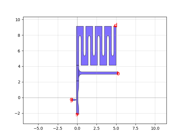
This code is a bit more concise, and nicely separates the arguments for the different sub-devices of the circuit: parameters for configuring the meander are passed in to qg.devices.snspd.basic when generating the meander_spec. Not only is the code easier to read, but it’s also much more maintainable and composable. Imagine we would like to tweak the design a bit to use the ntron.sharp geometry. With the ntron_meander_complicated implementation, we would need to write a whole new function or increase the number of arguments even more, or resort to using **kwargs, which makes code difficult to understand and document. Fundamentally the **kwargs pattern has problems when composing many functions due to the possibility of naming conflicts, and in general should be avoided except in situations where the input arguments to a function are unknown (e.g. in a decorator). 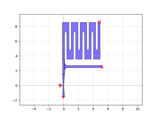By using the DeviceSpec pattern, to change the ntron type, we just pass a different DeviceSpec for the ntron_spec argument. For example:

ntron_spec = qg.devices.ntron.sharp
D = ntron_meander(ntron_spec, meander_spec, tee_spec, layer_spec=(1, 0))
qp(D)

Use of extend_ports

In order to avoid current crowding, optimal tapers should be used when transitioning from a narrow device to a wide routing trace. See Clem, J. & Berggren, K. “Geometry-dependent critical currents in superconducting nanocircuits.” Phys. Rev. B 84, 1-27 (2011). This can be achieved with phidl.geometry.optimal_step. Instead of manually instantiating and connecting these tapers, we can use functools.partial along with the extend_ports utility provided by qnngds to do this in a more concise way:

import qnngds as qg
import phidl.geometry as pg
from phidl import quickplot as qp
from functools import partial

taper = partial(pg.optimal_step, end_width=1, symmetric=True, layer=(1, 0))
snspd = qg.utilities.extend_ports(
    device=qg.devices.snspd.vertical(extend=None),
    port_names=(1, 2),
    extension=taper,
    auto_width=True,
)
qp(snspd)

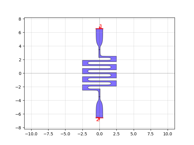
the auto_width argument to qg.utilities.extend_ports will ensure that the tapers automatically match the starting width of the SNSPD. This can be useful if the device whose ports you wish to extend has several ports with different widths; you can just specify the desired final width for routing and extend_ports will automatically create the necessary taper geometries.

Lithography test structures

Alignment markers

The alignment marks provided by qnngds.test_structures.alignment_mark and qnngds.test_structures.multilayer_alignment create vernier caliper comb(s) between two layers. This allows one to measure with an optical microscope sub-micron alignment errors. The design is written with photolithography in mind, given the large area. However, they can be adapted to be used to measure alignment between high and low-current e-beam exposure if the structures are appropriately outlined to limit the writing time.

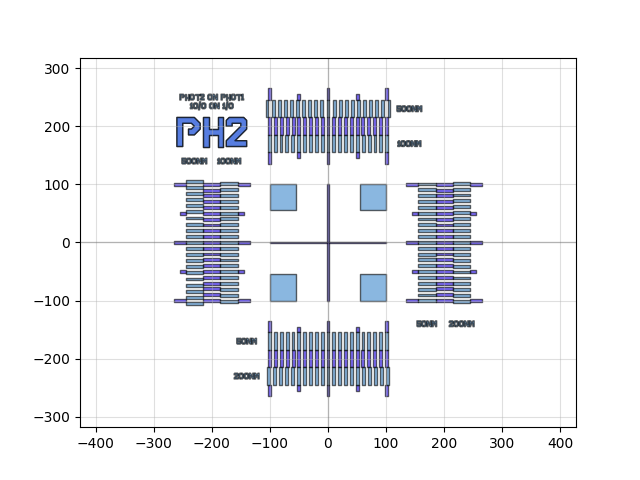
Usage:

1. Start by locating the calipers on the first layer (the central caliper).

2. Find the position where the calipers on each layer are aligned.

3. Count the number of positions between the center of the comb and the position at which the calipers are best aligned between the two layers.

4. Multiply the number from step 3 by the vernier offset (labeled next to the caliper).

5. For best accuracy, pick a caliper with a vernier offset such that best alignment occurs at > 5 positions away from the center.

6. Repeat for both vertical and horizontal calipers to determine the misalignment in each direction.

Resolution structures for dose-defocus tests

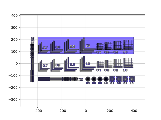
In order to calibrate the correct dose (and defocus for optical lithography), it’s useful to have a variety of lithographic test structures for analyzing failure modes for smaller features. The qnngds.test_structures.dose_defocus test structure provides a fairly comprehensive set of structures. Depending on the particular structure being fabricated, some structures may be more relevant than others. For example, for long wires, resolution_L and resolution_checkerboard may be most useful, whereas for dense features, resolution_waffle and resolution_checkerboard may be more useful. litho_stars can be helpful as well for non-manhattan oriented features, as well as for wires joining at a shallow angle.

Device arrays

phidl provides several methods for arraying devices. However, in some cases, one wishes to create a grid of identical devices. phidl.geometry.grid can achieve this, but it does not store/represent the array in the most efficient way. Furthermore, you lose access to the ports on the device after performing this operation.

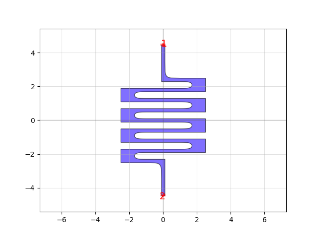
qnngds provides a special method for qnngds.Device instances, qnngds.layout.Device.add_array(). Lets say we want to make a linear array of identical SNSPDs and route them:

import qnngds as qg
from phidl import quickplot as qp
from functools import partial

snspd = qg.devices.snspd.vertical()
qp(snspd)

from qnngds import Device

D = Device("SNSPD array")
arr = D.add_array(
    device=snspd,
    columns=5,
    rows=1,
    spacing=(10, 0),
)

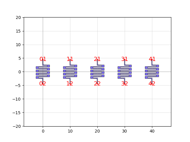
This leverages the gdspy primitve CellArray, which is an efficient way to store the layout Furthermore, we can access the ports like so:

for n, port_dict in enumerate(arr.ports[0, :]):
    for port_name, port in port_dict.items():
        D.add_port(name=f"{n}{port_name}", port=port)

Now, if we plot D, we can see the new ports we’ve added to it from the CellArray.

qp(D)

arr.ports[0, 0]