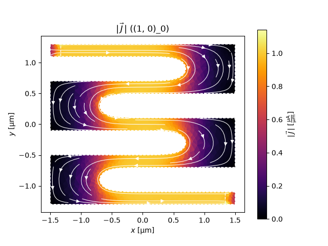
TDGL, London, and FEM normal-state analysis

In this set of tutorials, we will cover conversion of qnngds.Device to skfem.mesh.MeshTri1, tdgl.Device, and superscreen.Device for analysis of device properties.

First, let’s analyze a structure with femwell/skfem to visualize the current density of our device in the normal state.

import qnngds as qg
import matplotlib.pyplot as plt
from qnngds.analysis.fem import (
    make_mesh,
    solve_laplace,
    visualize_mesh,
    visualize_current,
)

snspd = qg.devices.snspd.basic(size=(3, 3))

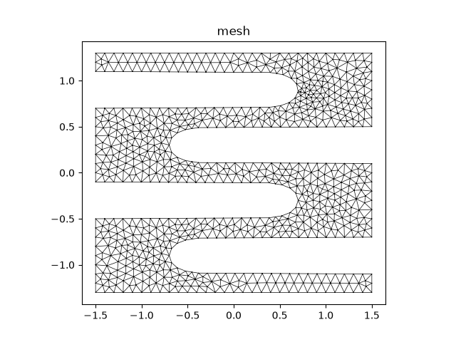
we can create a mesh as so:

mesh = make_mesh(device=snspd, layer=(1, 0), tolerance=0.01)
visualize_mesh(mesh)
plt.show()

Now, let’s analyze the current density by solving the laplace equation

result = solve_laplace(mesh)
visualize_current(result, ("1", "2"))
plt.show()

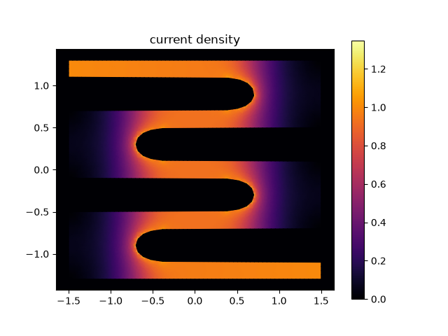
The current density is normalized to the current density at the excitation ports.

Next, we will show how to generate a tdgl.Device

from qnngds.analysis.tdgl import make_tdgl_device

device = make_tdgl_device(
    device=snspd,
    coherence_length=0.005,
    london_lambda=0.35,
    thickness=0.01,
    gamma=23.8,
    layer=(1, 0),
)
fig, ax = device.draw()
plt.show()

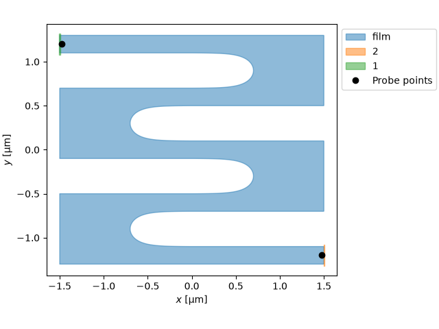
We can use this object to do tdgl simulations, check out the py-tdgl docs for more info and examples.

In some cases, we may be interested in modeling screening effects and Meissner currents in multi-layer structures. Note that py-tdgl can simulate screening, but is limited to a single layer. In order to simulate screening on multiple layers, we can use superscreen.

First, let’s create a gated diode device with a 5 nm thick layer having \(\lambda = 0.33\) μm penetration depth and a 40 nm thick layer having \(\lambda = 0.4\) μm penetration depth, separated by 45 nm spacer.

import superscreen as sc
from qnngds.analysis.superscreen import make_superscreen_device

qg.pdk.get_generic_pdk().activate()
diode = qg.devices.diode.gated(
    channel_spec=qg.devices.diode.basic(
        layer=(1, 0),
    ),
    gate_spec=qg.geometries.optimal_hairpin(
        width=1,
        pitch=3,
        layer=(10, 0),
    ),
)
scdev = make_superscreen_device(
    diode,
    london_lambda={(1, 0): 0.33, (10, 0): 0.4},
    thickness={(1, 0): 0.005, (10, 0): 0.04},
    z0={(1, 0): 0, (10, 0): 0.05},
    min_refine_points=1000,
)
fig, ax = scdev.draw(figsize=(6, 4))
_ = scdev.plot_polygons(ax=ax, legend=True)
plt.show()

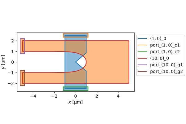
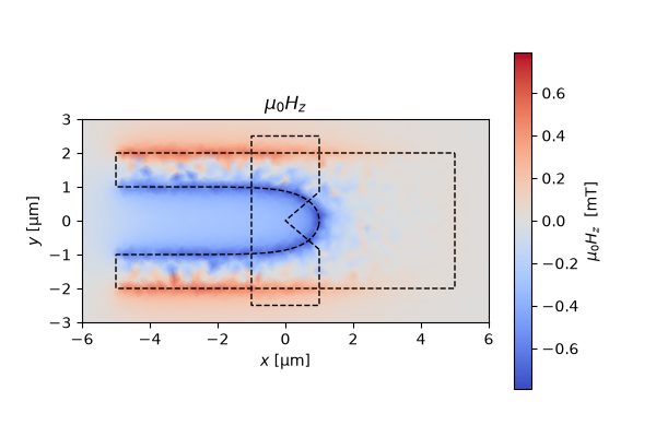
Now, we can simulate a 1 mA bias current flowing through the upper hairpin “gate”

Ibias = "1 mA"
scdev.make_mesh(max_edge_length=0.25)
solutions = sc.solve(
    scdev,
    terminal_currents={
        "(10, 0)_0": {"port_(10, 0)_g1": Ibias, "port_(10, 0)_g2": f"-{Ibias}"}
    },
    iterations=10,
    progress_bar=True,
)

Evaluating the solution at a distance of 10 nm (5 nm above the bottom film), we can plot the field distribution due to the current flowing through the upper layer.

eval_region = sc.Polygon(points=sc.geometry.box(12, 6))
eval_mesh = eval_region.make_mesh(min_points=2000)
fig, ax = solutions[-1].plot_field_at_positions(
    eval_mesh, zs=0.01, figsize=(6, 4), symmetric_color_scale=True, cmap="coolwarm"
)
for film in scdev.films.values():
    film.plot(ax=ax, color="k", ls="--", lw=1)
plt.show()

We can also use superscreen to compute the current density in a wire. Let’s reuse the same snspd device from earlier that we analyzed with femwell:

scdev = make_superscreen_device(
    device=snspd,
    london_lambda=0.33,
    thickness=0.005,
    min_refine_points=1000,
)
scdev.make_mesh(max_edge_length=0.25)
Ibias = f"{snspd.ports[1].width} uA"
solutions = sc.solve(
    scdev,
    terminal_currents={
        "(1, 0)_0": {"port_(1, 0)_1": Ibias, "port_(1, 0)_2": f"-{Ibias}"}
    },
    iterations=10,
    progress_bar=True,
)
fig, ax = solutions[-1].plot_currents(films=["(1, 0)_0"])
_ = scdev.plot_polygons(ax=ax[0], color="w", ls="--", lw=1)
plt.show()